入黎免費幫你砌excel表 / 教你formula (8)

用 google sheets + apps script

呢個再click入去Transform Data就係Power Query
可以set返d column format

都得
不過好少用Apps Script
有用開Office Scripts都係JS但有少少唔同

因為我要配合射上web ，所以選擇學 apps script

https://hkspd.siuyeong.com

我想請教各位Ching
點樣可以整formula排sequence?

Example
Sequence 係 A>B>C>D


123 A
123 B
123 C
456 C
456 D
789 B
789 D


Result
123 A
456 C
789 B

你 Example 係 A>B>C>D
但你 show 嘅 Result 係 A>C>B

就算佢排岩呢個都唔係叫排sequence
好彩佢有example
如果佢冇example我會完全諗左另一樣野

btw, 我發覺 Google Sheets 好似齊晒 365 啲 func. 唔洗煩 excel 版本問題

但google sheet係browser 上面用始終冇咁順手
同埋googlesheet有啲function個behaviour 同excel唔同

雙修達人

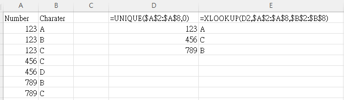
呢種唔係排Sequence, 只係抽出column a既unique 值, 再拎第一個column b既值去做西選

excel傳心師

痴線, 點解會明

我見到佢有開post問　

https://lihkg.com/thread/3170983/page/1

笑死

我睇完個POST之後發現其實唔係想要我整左既果D野 而且睇完之後更加唔明

以為你傳心成功

求救Microsoft 365版本

我而家有以下既excel data
Column A; Column B; Column C; Column D-O; Column P
Product; sales channel; Indicator; January - December; Total
Apple; supermarket; Quantity; 一月至12月既銷量; 成個row既total
Apple; supermarket; Revenue; 一月至12月既revenue; 成個row既total
Apple; supermarket; Cost; 一月至12月既買貨成本; 成個row既total
Apple; online; Quantity; 一月至12月既銷量; 成個row既total
Apple; online; Revenue; 一月至12月既revenue; 成個row既total
Apple; online; Cost; 一月至12月既買貨成本; 成個row既total
Apple; total channel; Quantity; 一月至12月既銷量; 成個row既total
Apple; total channel; Revenue; 一月至12月既revenue; 成個row既total
Apple; total channel; Cost; 一月至12月既買貨成本; 成個row既total
假設我有成千種類既貨物係以下既row
而最後三個row分別係1月至12月既所有產品在所有channel既total quantity, total revenue and total cost

而家想整一個pivot chart (折線圖), 想show x axis係1-12月, y axis係quantity, 然後想filter某一個產品(例如apple既quantity同埋total所有產品既quantity整成兩條折線, 應該點樣set pivot table fields果4個格仔試極都唔岩

問題係你1-12月係column field名
正常應該係有個column做month，data rows有1-12月
首先你要用power query unpivot左d data先

https://youtu.be/ESap6ptV8fI
有咩唔明再問

留名學野

呢張同上面張手機留名圖都高登年代既野, 估唔到仲有人用好懷念